A live Bayesian estimate of Brazil’s 2026 runoff and the identifiability of an order-of-counting term
This post records the methodology of a small Bayesian model that followed Brazil’s 2026 presidential runoff on 25 October, from the eve polls to the final count. It gives the data flow and the full formulation of the model, the three changes made to it while the count was running and how each version compares with the final result. The comparison is useful for anyone who runs a model on live partial data, because one of the changes illustrates a general issue, a term that cannot be identified from the data available at the moment it is used.
Data flow
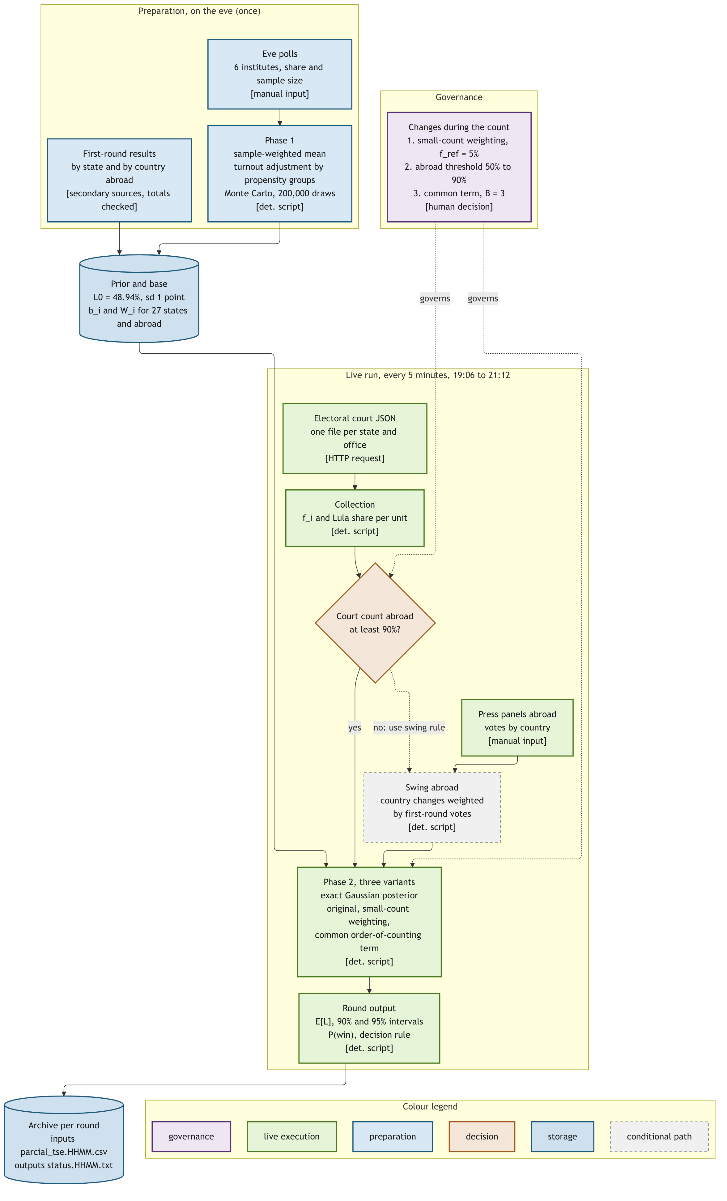
Two inputs are fixed before the count starts. The eve polls feed phase 1, which produces the national prior, and the first-round results by state and by country abroad give, for each unit, the baseline share and the weight. During the count, a collection script reads the electoral court’s official JSON files, one per state and per office, and extracts for each unit the share of the electorate already counted and Lula’s share of the two finalists’ votes. The court’s count abroad arrives in blocks by continent, so until it covers 90% of the vote abroad, that unit enters through a swing computed country by country from press panels. Phase 2 then computes the posterior in three variants, and each round’s inputs and outputs are archived, which is what allows the scores and the decomposition below to be recomputed.
Formulation
Phase 1, the eve prior
Six eve polls j, with Lula’s share of valid votes L_j and sample size n_j, are combined by sample size,
\bar L = \frac{\sum_j n_j L_j}{\sum_j n_j} = 49.33\%.
The turnout adjustment splits the electorate into two propensity groups with shares \pi_A = 0.76 and \pi_B = 0.24 and Flávio Bolsonaro shares F_A = 52\% and F_B = 48\%. With turnout rates t_A and t_B, group B’s share among voters is w = \pi_B t_B / (\pi_A t_A + \pi_B t_B), and the shift in Flávio Bolsonaro’s share relative to the electorate is
\Delta(t_A, t_B) = \big[(1 - w) F_A + w F_B\big] - \big[\pi_A F_A + \pi_B F_B\big].
The point prior is L_0 = \bar L - \Delta(0.95, 0.50) = 49.33 - 0.39 = 48.94\%. The Monte Carlo draws t_A \sim U(0.85, 0.98), t_B \sim U(0.30, 0.90), a poll error \varepsilon \sim N(0, 1) and a rounding term \rho \sim U(-0.5, 0.5)/\sqrt{2} for the two polls published with rounded shares, and computes L^{(k)} = \bar L - \Delta(t_A^{(k)}, t_B^{(k)}) + \varepsilon^{(k)} + \rho^{(k)}. Over 200,000 draws, P(L > 50) = 0.178.
Phase 2, state space
There are n = 28 units, the 27 states and voters abroad. For unit i, b_i is Lula’s share of the two finalists’ votes in the first round and v_i its first-round valid votes, with weights W_i = v_i / \sum_k v_k. Lula’s runoff share in unit i and nationally are
p_i = b_i + s + u_i, \qquad L = \sum_i W_i\, p_i,
where s is the national swing and u_i the unit’s own deviation. In the variant with the common order-of-counting term, the state is
x = (s, u_1, \dots, u_n, \beta)^\top \sim N(m_0, C_0),
m_0 = (s_0, 0, \dots, 0, 0)^\top, \qquad C_0 = \mathrm{diag}(\sigma^2, \tau_1^2, \dots, \tau_n^2, B^2),
with \sigma = 1, \tau_i = 2 for states and 5 abroad, B = 3, and s_0 = L_0 - \sum_i W_i b_i = +0.16, so that the prior mean of L equals the phase-1 prior. The other two variants are the same model without \beta. With no counts, L has mean 48.94\% and standard deviation 1.155 points, and P(L > 50) = 0.179.
Each partial count y_i, Lula’s share of the two finalists’ votes among the ballots counted so far, is an observation
y_i = b_i + h_i^\top x + e_i, \qquad h_i = \mathbf{e}_s + \mathbf{e}_{u_i} + \lambda_i\, \mathbf{e}_\beta, \qquad e_i \sim N(0, r_i^2),
where \mathbf{e} denotes a coordinate vector, \lambda_i = 1 - f_i for counts from the court, \lambda_i = 0 for the swing rule abroad, and f_i is the share of the unit’s electorate already counted. The noise is
r_i = \kappa(1 - f_i) + 0.1 \quad \text{(original)},
r_i = \frac{\kappa(1 - f_i) + 0.1}{\sqrt{\min(1, f_i / f_{ref})}} \quad \text{(small-count weighting)},
with \kappa = 4 and f_{ref} = 0.05. Under the swing rule, voters abroad enter as y_{ZZ} = b_{ZZ} + \hat\delta, with
\hat\delta = \frac{\sum_c \omega_c \big(q^{(2)}_c - q^{(1)}_c\big)}{\sum_c \omega_c}, \qquad \omega_c = v^{(1)}_c \min\!\Big(1, \frac{v^{(2)}_c}{v^{(1)}_c}\Big),
where q^{(1)}_c and q^{(2)}_c are Lula’s two-finalist shares in country c in the first round and in the runoff partial, v^{(1)}_c and v^{(2)}_c the corresponding votes, and f_{ZZ} = \sum_c \omega_c / \sum_c v^{(1)}_c.
Each round starts again from (m_0, C_0) and absorbs the latest partial of each unit, one at a time,
S = h_i^\top C h_i + r_i^2, \qquad K = \frac{C h_i}{S},
m \leftarrow m + K\big(y_i - b_i - h_i^\top m\big), \qquad C \leftarrow C - K h_i^\top C.
Since the model is linear and Gaussian and each unit contributes one observation per round, the result is the exact posterior and does not depend on the order of the updates. With a = (1, W_1, \dots, W_n, 0)^\top, the national share has posterior
\mathbb{E}[L] = \sum_i W_i b_i + a^\top m, \qquad \mathrm{sd}(L) = \sqrt{a^\top C a},
P(\text{Lula wins}) = \Phi\!\left(\frac{\mathbb{E}[L] - 50}{\mathrm{sd}(L)}\right),
with 90% and 95% intervals \mathbb{E}[L] \pm 1.645\,\mathrm{sd}(L) and \mathbb{E}[L] \pm 1.96\,\mathrm{sd}(L).
Decision rule
With \ell and \varphi the votes already counted for each finalist, the votes still to be counted are estimated as
R = (1 + M) \Big[\sum_{i\ \text{counted}} (1 - f_i)\, v_i + \sum_{i\ \text{not counted}} v_i\Big], \qquad M = 0.10,
and the race is declared when |\ell - \varphi| > R. An absolute version replaces R with eligible voters minus votes counted. The rule needs a counted share of at least 1.1/(1.1 + m) for a final margin of m points.
Three changes made during the count
Down-weighting small counts. Under the original noise rule, a state with 0.02% of its electorate counted had almost the same weight on the national swing as a state with 50% counted, since \kappa(1 - f) + 0.1 barely moves between those two values. The first ballots are not a random sample, so the change replaces the original r_i with the small-count version above, which is identical for f_i \ge f_{ref}. With 0.21% of the national electorate counted, the original model gave a Lula win a probability of 0.664, and the down-weighted version gave 0.217, close to the eve value.
Extending the swing rule for voters abroad. By 19:02 the court had counted 60% of the vote abroad, almost all from Europe and Asia, with Lula at 59.7%. Without the Americas, that partial was not representative of the vote abroad and was moving the national swing. The threshold for using the court’s count abroad went from 50% to 90%, and the swing rule was used until then.
A common order-of-counting term. Within several states, Lula’s share was falling as the count advanced, from 43.8% to 39.6% in Mato Grosso and from 73.5% to 69.9% in Paraíba, which suggested that the earliest ballots, often from state capitals, deviated in the same direction across states. Without \beta, such a common deviation is attributed entirely to s. The change adds \beta \sim N(0, B^2) to the state, with loading \lambda_i = 1 - f_i, so that its contribution fades as each state’s count completes. At 19:28, with under 5% of the electorate counted, this version gave a Lula win a probability of 0.306, against 0.991 for the down-weighted version. From 19:33 on it was used as the main version. The value of B was set by judgment during the night.
Results
The count paused at 17:06 and resumed at about 19:02. At the first round of updates after the restart, at 19:11, the raw national share was 52.1%. It fell below 50% at 19:50, reached 49.53% at 20:01, rose above 50% again at 20:28 and finished at 51.75%, with 64,060,863 votes for Lula and 59,720,297 for Flávio Bolsonaro. The main version’s final estimate was 51.72%, with a 95% interval from 51.66% to 51.79%, and its decision rule declared the race at 21:12, with a margin of 4.33 million votes against 363,000 still to be counted. The national swing over the first round, as estimated by the model at the end of the count, was about +2.4 points, while the eve polls implied +0.16.
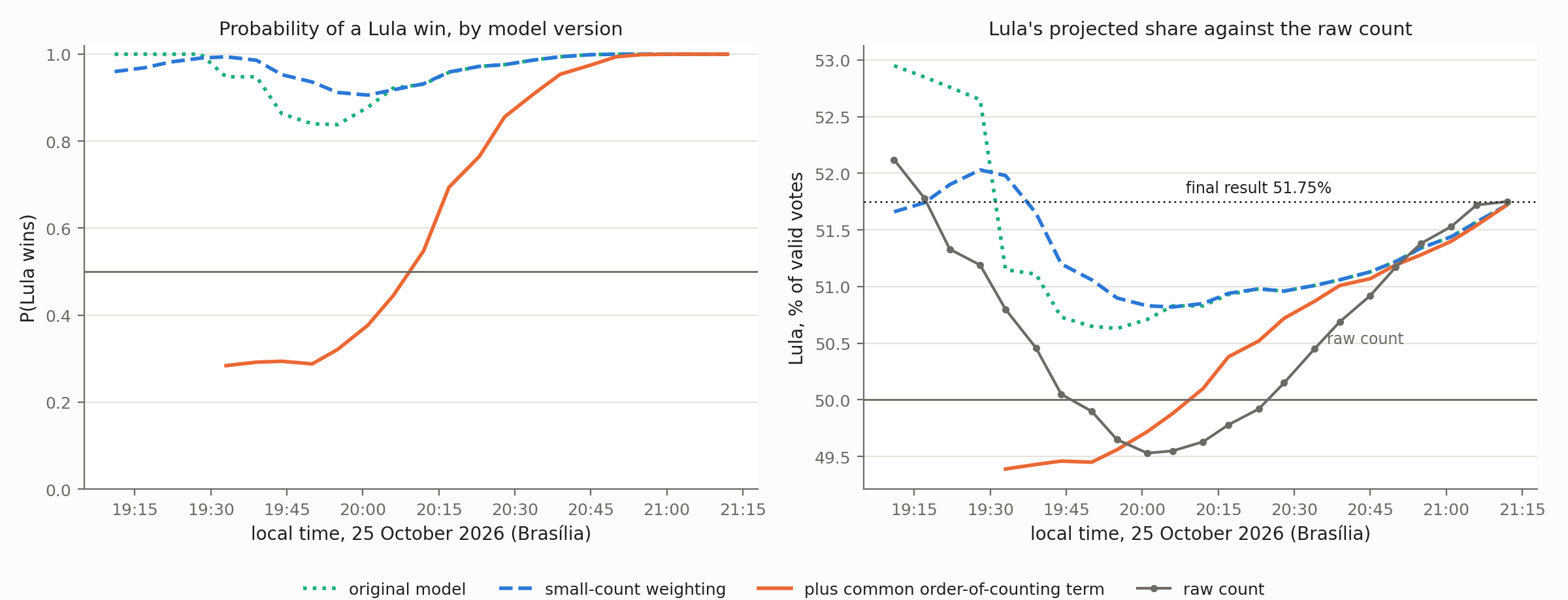
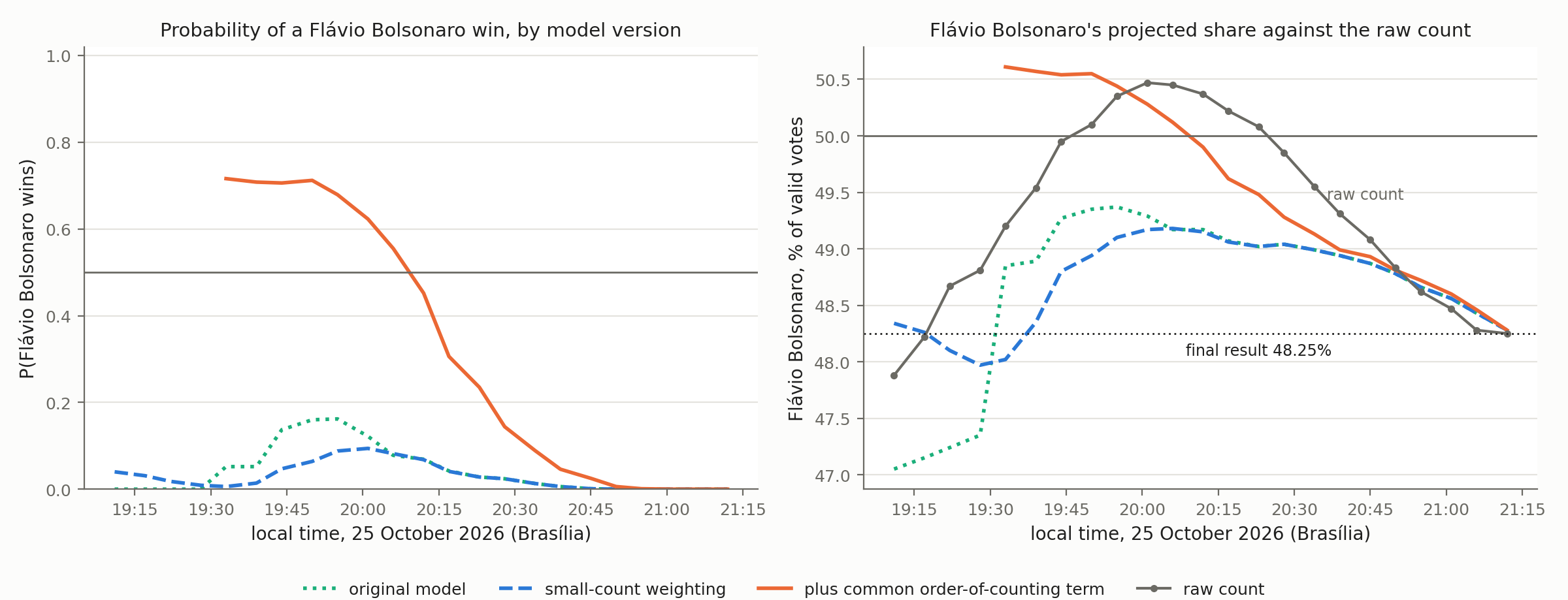
Between 19:33 and 20:06, the version with the common term gave a Lula win a probability between 0.28 and 0.45, while the two versions without it gave between 0.84 and 0.99. The table compares the three versions with the final result over the 19 rounds in which all three were running. Lower values are better in the first three columns.
| Version | Brier score | Log score | Mean absolute error of \mathbb{E}[L] | Rounds with P < 0.5 for the winner |
|---|---|---|---|---|
| Original | 0.0055 | 0.053 | 0.70 pt | 0 |
| Down-weighting small counts | 0.0020 | 0.031 | 0.58 pt | 0 |
| Plus common order-of-counting term | 0.1874 | 0.497 | 1.29 pt | 7 |
In the race for governor of the Federal District, followed with the same model as a single unit, prior 39.76% for Leandro Grass with \sigma = 4 and \tau = 0, Celina Leão received 57.2% of valid votes and Leandro Grass 42.8%, and the decision rule declared the result at 20:01, with 89% counted.
Identifiability of the common term
The common term was intended to separate two components that look alike early in the count. One is a deviation of the first ballots from the final result, which fades as the count completes. The other is the national swing, which does not. In the observation vector h_i, they differ only through the loading \lambda_i = 1 - f_i. When every state has a small share counted, \lambda_i \approx 1 for all i, so the coordinates of s and \beta enter every observation with almost the same coefficient. The data then carry little information about how to divide a common deviation between them, and the posterior divides it roughly in proportion to their prior variances, B^2 = 9 for \beta and \sigma^2 = 1 for s.
Re-running the main version on the archived partial counts shows the division. At 19:34, the common term held +5.10 points, the national swing had moved from +0.16 to +0.82, and the posterior correlation between the two was −0.69. At 20:12, the common term held +2.00 and the swing +1.62. At 21:12, with the count complete, the common term was −0.02 and the swing +2.39. During the first hour, most of the common deviation was attributed to \beta, which kept \mathbb{E}[L] close to the eve prior, and the attribution moved to s as the counts accumulated and the loadings 1 - f_i fell.
The pattern of early deviations was also not uniform in sign. Early ballots favoured Lula relative to the final state result in the North and Centre-West, with Mato Grosso going from 43.8% to 33.7% over the night, and favoured Flávio Bolsonaro in São Paulo and Rio Grande do Sul, with São Paulo going from 38.8% to 46.1%. A single common term with a single sign cannot represent both patterns.
These comparisons rest on a single outcome. The scores are computed over 19 rounds of the same event, which are strongly dependent, and they do not establish that one version is better calibrated than another in general. A version can assign high probability to the eventual winner without being better calibrated. What a single night can show is whether each component behaved as designed. The down-weighting of small counts kept the estimate near the prior until the counts carried more information. The common term could not be separated from the national swing during the period in which it carried most weight.
Open points
- The value B = 3 and the sign structure of the order-of-counting term require calibration against an archived count, the 2022 runoff being a natural candidate. A version with one term per region, or one estimated from the within-state trajectories of the count rather than from the cross-state common deviation, would be able to represent the pattern observed here.
- The decision rule required a counted share of about 97% for the final margin of 3.5 points, which is why the declaration came at 21:12. Its absolute version includes abstentions in the votes still to be counted and is not reached in practice.
- The country-level first-round file used for voters abroad has duplicated rows, and one press panel reported numbers for the United Kingdom that conflict with another source. Neither affects the national result, since voters abroad were 0.28% of the first-round valid vote.
- The official JSON files contain everything the model needs by state and by office and can be read with a plain HTTP request, which press dashboards did not allow.
For models updated on live partial data, the practical point is to check, before adding a term that absorbs a pattern, whether the data available at the time of use can identify it. When the term and the quantity of interest enter the same observations with nearly the same coefficients, their prior variances determine how a common deviation is divided between them.
Source. Own model and own run, with partial counts from the official JSON files of Brazil’s electoral court (resultados.tse.jus.br), read every five minutes on 25 October 2026. Scores, the eve probabilities and the posterior decomposition were recomputed from the model code and the archived inputs and outputs of each round.
I write about this kind of work, scientific method, statistics, and AI applied with rigor, on LinkedIn: linkedin.com/in/pcbrom.