The same quantization recipe, three different verdicts
“Quantization preserves quality” circulates as though it were a property of the method. It is not. It is an empirical result, and results are conditional. Here is the same recipe, int4 quantization-aware training, run against three local models and evaluated with the same paired test on the same seeded problems. It produces three different verdicts.
The three verdicts
All comparisons run with reasoning off, at n = 120, on multi-step arithmetic with the gold computed in Python, scored with an exact McNemar test on the paired items (McNEMAR, 1947).
| int4 QAT build | Comparator | Accuracy | McNemar p | Verdict |
|---|---|---|---|---|
e2b-it-qat |
e2b (its own original) |
0.3000 vs 0.2833 | 0.82 | no detectable difference |
26b-a4b-it-qat |
26b-fast (PTQ Q4_K_M) |
0.6833 vs 0.7833 | 0.012 | worse |
31b-it-qat |
26b-fast (PTQ Q4_K_M) |
0.8917 vs 0.7833 | 0.024 | better |
Read the third row before drawing any conclusion from the second.
On the e2b pair the quantized variant is indistinguishable from the original, 40 percent smaller on disk and about 4 percent faster. Same quality, less memory, marginally more throughput. Approved.
On the 26b-a4b pair the identical recipe loses ten points and the test rejects at p = 0.012. Rejected.
And then there is the dense 31b-it-qat, which is also an int4 QAT build, and which is the strongest model in the entire study: 0.8917, beating the post-training-quantized 26b-fast by a significant margin (p = 0.024, with 21 items correct only for the 31B against 8 only for the 26B).
That third row does real work. It kills the simple story. If int4 QAT degraded quality as a technique, the dense QAT model would not be the best thing on the machine. It is. So whatever went wrong in the middle row is not “QAT is lossy”. It is something about that particular model, or about how it was compared, and the next section is about not pretending to know which.
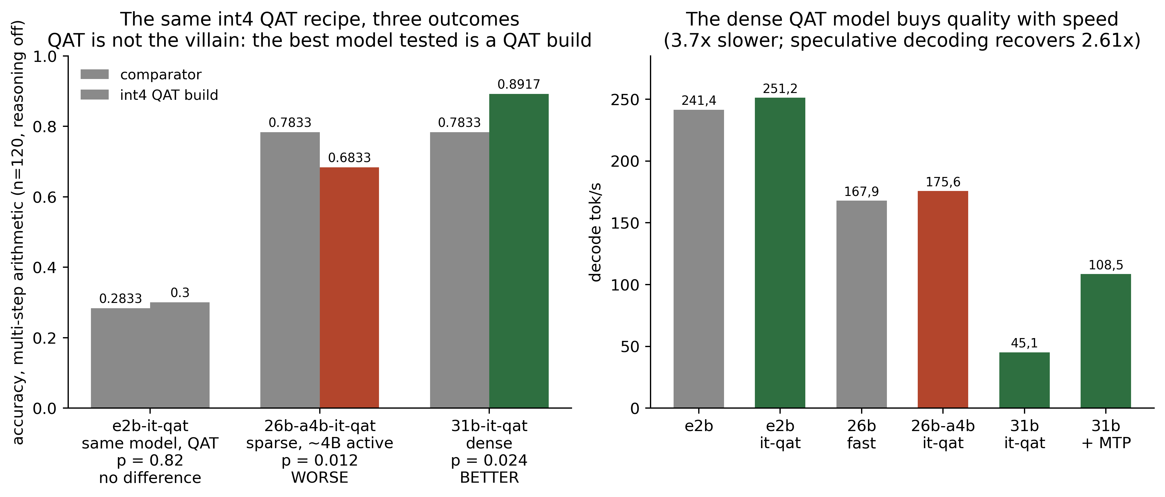
Note what the right-hand panel says, because it is the reason this trap is easy to fall into. The quantized variants are smaller and slightly faster, in both families, exactly as advertised. Every metric that is cheap to measure looks fine. The one that is expensive to measure, quality under a paired test in the regime you actually deploy, is the one that separates the verdicts.
| Variant | decode tok/s | Size |
|---|---|---|
e2b (original) |
241.4 | 7.2 GB |
e2b-it-qat |
251.2 | 4.3 GB |
26b-fast (PTQ Q4_K_M) |
167.9 | 17 GB |
26b-a4b-it-q4_K_M |
168.5 | 17 GB |
26b-a4b-it-qat |
175.6 | 15 GB |
31b-it-qat (dense) |
45.1 | 19 GB |
31b-it-qat + speculative decoding |
108.5 | 19 GB |
The dense QAT model is the quality choice and it is not free: at 45.1 tok/s it decodes roughly 3.7 times slower than the sparse family, because a dense forward pass computes all 31B parameters per token while the sparse one activates about 4B. Speculative decoding recovers most of that, lifting it to 108.5 tok/s, a 2.61x speedup, without changing the output. Quality, speed, memory: you get to pick, and the picking is the whole job.
The confounders, which are mine to declare
Two of them, and neither is optional to state.
The prompt template. The two variants in the failing pair differ in two ways at once: the quantization method, int4 QAT against post-training Q4_K_M, and the prompt template, since one variant carries an explicit template and the other uses the native renderer. A template difference can move accuracy on its own. To attribute the drop to quantization alone, the run has to be repeated with an identical template on both sides, and that has not been done.
The architecture. This is the one I got wrong first, and it is the reason the section above refuses the word “bigger”. The failing pair is not simply a larger version of the passing pair. The 26b-a4b family is sparse: it carries 26B parameters but activates only about 4B of them per token. The e2b family is a different architecture at a different scale. So the two pairs differ in how many parameters actually participate in each forward pass, not just in how many exist.
That distinction matters because there is a mechanism attached to it, and because the third row of the table points at it. In a sparse model, each active weight carries proportionally more of the computation, and the routing that selects which experts activate is a discrete decision that quantization noise can flip. A quantization budget that is harmless when spread across a dense forward pass is not obviously harmless when concentrated on a small active subset.
Notice that the evidence leans this way. The two models that took int4 QAT without damage are the dense 31B, which is the best model in the study, and the small e2b. The one that took damage is the sparse one. That is suggestive, and it is not proof: it is three models, the failing comparison also carries the template difference, and the 31B is measured against a different model rather than against its own unquantized self. I am reporting the pattern, not closing the case.
So the honest statement is narrower than the headline. What is established: the shipped 26b-a4b-it-qat build is worse than 26b-fast in the reasoning-off regime, and int4 QAT is not degrading quality as a general matter, because the strongest model here is a QAT build. What is not established: why the sparse one broke. Sparsity and template are confounded in that comparison, and separating them takes a run with an identical template that has not been done.
I state this because a result that hides its author’s confounders is not usable by anyone, including its author. It also does not rescue the practical conclusion, which survives every explanation on offer: whatever the mechanism, that build is worse in the regime it would run in, and that is the decision the benchmark exists to inform.
A final limit, for completeness: a logit-level divergence check, which would give a mechanism-level read rather than an outcome-level one, was not available in this environment, so the evidence here is entirely behavioural.
What transfers
Do not inherit a quantization verdict. Not from another model, not from another architecture, not from another inference regime. Three models took the same recipe here and landed in three different places, and the one that broke is not the one a size heuristic would have predicted.
The heuristic that fails is “bigger models absorb quantization better”. The heuristic that survives, tentatively, is that a model with few active parameters per token has less redundancy to spend on a degraded weight representation. Even that one you should not take from me. You should measure it on your model, in the regime you deploy.
The cost of measuring is one seeded evaluation set and one paired test. The cost of not measuring is a silent ten-point regression in the configuration you ship.
Source. Own measurement, RTX 4090, local inference, temperature zero, reasoning off. Multi-step arithmetic generated with a seed, gold computed in Python, identical items across models, exact paired McNemar. Throughput measured over repeated generations at fixed output length.
Reference. McNEMAR, Q. Note on the sampling error of the difference between correlated proportions or percentages. Psychometrika, v. 12, n. 2, p. 153-157, 1947. DOI: 10.1007/BF02295996.