gpumetropolis 0.4: a guided tour of a Bayesian toolkit that declares where it loses
A sampler becomes a tool the day you can answer a question with it end to end, from the fit to the decision to the picture that convinces a reader. Version 0.4 of gpumetropolis is where the package crosses that line. It adds a sampler for correlated targets, an information-bound reference that knows when to stay silent, the decision and model-comparison verbs that applied work needs, and three case studies on real data that exercise the whole thing. This post is the guided entry to that material, a reference to consult rather than an argument to read once: each tool gets one worked figure and a pointer to the full vignette shipped with the package on r-universe. The spine that holds it together is the benchmark, because the honest claim of this release is not that the package wins everywhere. It is that it tells you where it loses.
Differential Evolution: correlation without tuning
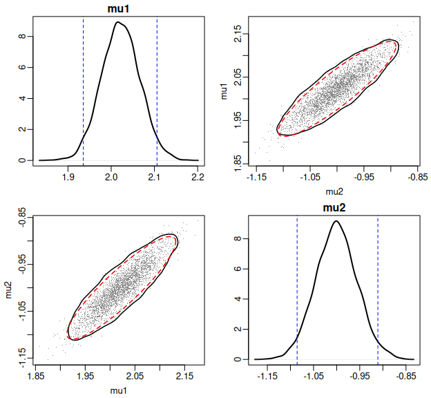
A random-walk sampler on a correlated posterior is slow for a mechanical reason: its proposal is round while the target is a thin diagonal ridge, so most steps push against the ridge and get rejected. The usual fix is to hand the sampler a tuned proposal covariance, which you rarely know in advance. Differential Evolution MCMC removes the tuning (TER BRAAK, 2006). It runs an ensemble of chains and proposes, for each one, the scaled difference of two others: x_c + gamma * (x_a - x_b) + epsilon. The difference of two draws from the target already carries the target’s correlation, so the proposal aligns with the ridge on its own, with no covariance to set. In gpumetropolis it is one argument, method = "de", and it maps onto the chain axis the package already parallelises.
The Cramer-Rao reference, and the refusal
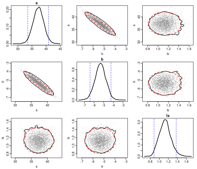
A fit should be read against a reference. The Cramer-Rao bound is the smallest variance any unbiased estimator can attain, set by the Fisher information (RAO, 1945; CRAMER, 1946); gpum_crlb() forms it from the observed information and reports it next to the posterior spread. On a regular model the two agree: on the mtcars regression the bound on the slope matches the standard error of lm() to the third decimal, and on the Port Pirie Gumbel fit it matches the standard error of evd::fgev. The reference earns its place precisely by knowing when it does not apply. Fit a two-component mixture to the Old Faithful geyser, where the posterior is genuinely multimodal because the component labels can swap, and gpum_crlb() refuses to report a number rather than print a misleading one, flagging the high split R-hat instead. A reference that answers every time is not a reference; it is a number generator.
The decision layer: from the posterior to a verb
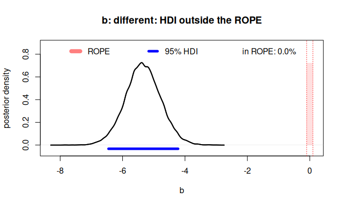
Inference ends in a decision, and the package gives the decision its own verbs, read straight from the draws. gpum_hypothesis() returns the posterior probability of a directional claim, hdi() the highest density interval, and gpum_rope() decides against a region of practical equivalence, a band of values too small to matter, in the style Kruschke set out (KRUSCHKE, 2018). On the mtcars slope the question is whether heavier cars are meaningfully less economical: the posterior probability that the slope is negative is effectively one, the 95% interval runs from -6.45 to -4.22 mpg per 1000 lb, and against a region of plus or minus a tenth of an mpg the entire interval sits outside it, so the decision is “different”, not merely “nonzero”.
The comparison layer: prediction and evidence are different questions
When a second predictor is on the table, two honest questions pull apart. Does it predict better out of sample, and does the data carry evidence for it under a stated prior? The package answers each with the right instrument. WAIC (WATANABE, 2010) and PSIS-LOO (VEHTARI; GELMAN; GABRY, 2017) score out-of-sample predictive accuracy from the pointwise log-likelihood, no marginal likelihood required; the lower value predicts better. The Bayes factor weighs the evidence, and its marginal likelihoods are estimated by thermodynamic integration (GELMAN; MENG, 1998), the path-sampling route between the prior and the posterior. On mtcars, adding horsepower to weight lowers the WAIC from 166.5 to 157.2, so it predicts better, and the Bayes factor reports substantial evidence for the richer model. The two need not agree in emphasis, because the Bayes factor is prior-sensitive in a way the predictive criteria are not (KASS; RAFTERY, 1995); reading them together, and reporting the prior, is the honest summary. The interpretation scale itself is old (JEFFREYS, 1961), and so is the warning that the factor moves with the prior even when the data do not.
Posterior predictive checks: the picture behind the number
A criterion is a scalar; the eye wants the distribution. gpum_ppc() draws a posterior predictive sample given the family’s one-line simulator, and gpum_density_compare() overlays the observed density against the generated ones. When two models generate almost the same distribution, as the two mtcars regressions do, the overlay shows why the eye cannot rank them and the predictive criteria must. When they do not, the picture carries the verdict on its own, which is the Port Pirie case below.
A worked deliverable: the hundred-year sea level
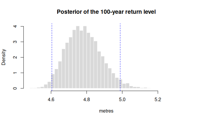
The point of a toolkit is a finished answer. The Port Pirie series is 65 annual maximum sea levels, the textbook extreme-value dataset (COLES, 2001). Extreme-value theory says the annual maximum of a long record follows a Gumbel law, and the engineering deliverable is the return level: the height exceeded on average once a century. Because every posterior draw of the location and scale gives one draw of the return level, its posterior comes for free, with an honest interval rather than a point. The hundred-year level comes out at 4.78 metres, with a 95% interval from 4.60 to 4.99. The choice of law is not free either: against a Normal fit to the same maxima, the Gumbel has the lower WAIC and LOO, because the right-skew of the extreme-value law matches the upper tail the return level actually reads.
The honest benchmark
Here is the spine. Run the same fit through gpumetropolis and the established samplers, and read two things: whether they agree on the answer, and what each costs. On all three cases they agree. Every sampler recovers the same regression slope near the least-squares value, the same Gumbel location near 3.87 metres; the comparison is about cost, not correctness. So the only honest axis is effective sample per second, computed uniformly with coda so the estimator is not a confounder.
On a small data set fit with a single chain, gpumetropolis does not lead, and the package says so. On the mtcars regression the conjugate Gibbs sampler of MCMCpack delivers around 1.25 million effective draws per second against the package’s roughly 15 thousand, with Stan near 10 thousand and nimble near 90, dragged down by the seconds it spends compiling a tailored sampler. On the Port Pirie Gumbel, where MCMCpack has no canned model, Stan’s gradient sampler leads at about 53 thousand, the generic mcmc random walk follows at 42 thousand, and gpumetropolis sits at 20 thousand. A tuned single-chain sampler on a small regular model is not the regime this package claims.
Its regime is the other one: many chains on an expensive log-density. There the registered benchmark records gpumetropolis reaching tens to hundreds of times the effective sample per second of the same competitors, the only one to scale to thousands of chains, from one formula that runs on CPU, CUDA and Vulkan. And even there the honest figure shows a loss: across the four target models at 64 chains, the package leads on the first three and nimble takes the fourth.
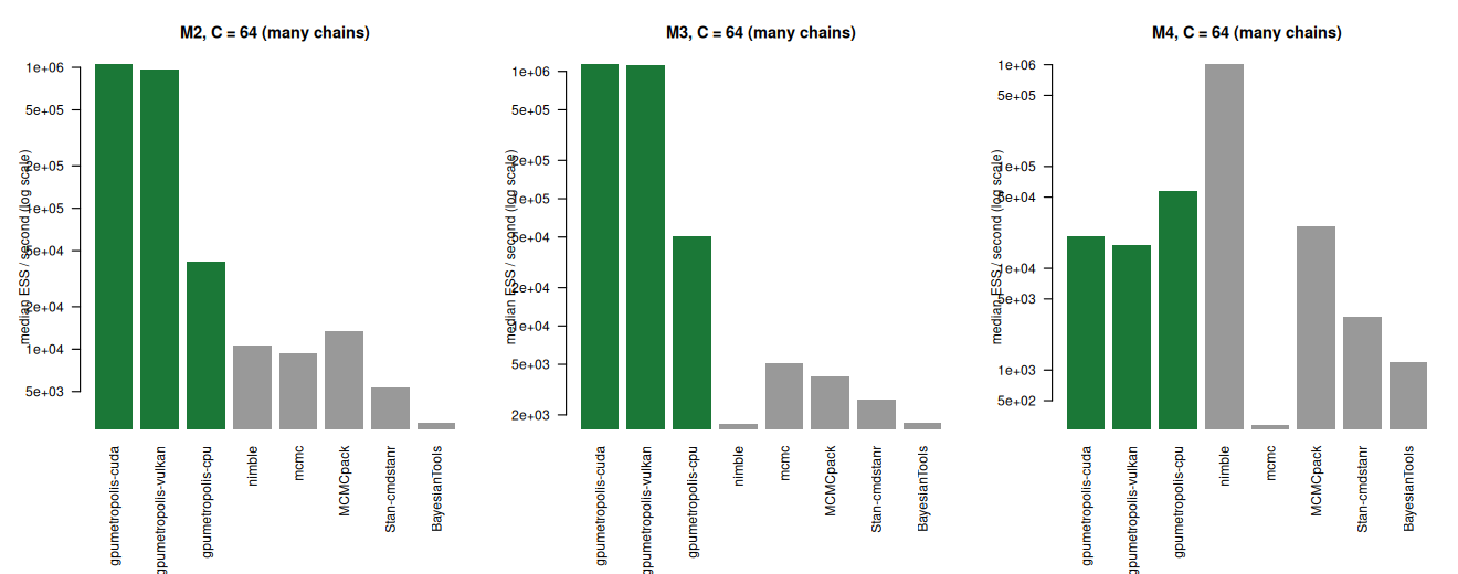
That is the release’s one claim, made twice, in code and in the chart: a package worth trusting names the regimes where it loses. MCMCpack owns conjugate regression, Stan owns smooth high-dimensional targets after a compile, nimble owns a long run where its compile cost amortises. gpumetropolis owns the many-chains, expensive-density corner, and is one formula away on a non-standard density that the canned packages cannot fit at all.
Where the scalar language stops
The same honesty applies to the package’s own edge. The full generalised extreme-value law adds a shape parameter that the Gumbel fixes at zero, and the classical Port Pirie question is whether that shape differs from zero. The package does not fit the generalised law here, because its log-density has a term singular at exactly the value the data sit near, and the scalar formula language cannot yet express the conditional that selects the Gumbel-limit branch. That is a named limit on the roadmap, not a gap left quiet.
How to read the rest
Each section above is one figure from a longer worked chapter. The three case vignettes, Old Faithful, mtcars and Port Pirie, and the two Differential Evolution vignettes run every tool end to end with its code and output, and they live with the package on r-universe. Read this post for the map; open the vignettes for the worked territory.
Source. gpumetropolis 0.4.0 and 0.4.1, released 2026-06-29 on r-universe; NEWS.md and the case vignettes case_old_faithful, case_mtcars, case_portpirie, demc_correlated and demc_banana. Figures are the package’s own rendered vignette and benchmark figures.
References
COLES, S. An Introduction to Statistical Modeling of Extreme Values. London: Springer, 2001. DOI: 10.1007/978-1-4471-3675-0.
CRAMER, H. Mathematical Methods of Statistics. Princeton: Princeton University Press, 1946. DOI: 10.1515/9781400883868.
GELMAN, A.; MENG, X.-L. Simulating normalizing constants: from importance sampling to bridge sampling to path sampling. Statistical Science, v. 13, n. 2, p. 163-185, 1998. DOI: 10.1214/ss/1028905934.
JEFFREYS, H. Theory of Probability. 3. ed. Oxford: Oxford University Press, 1961.
KASS, R. E.; RAFTERY, A. E. Bayes factors. Journal of the American Statistical Association, v. 90, n. 430, p. 773-795, 1995. DOI: 10.1080/01621459.1995.10476572.
KRUSCHKE, J. K. Rejecting or accepting parameter values in Bayesian estimation. Advances in Methods and Practices in Psychological Science, v. 1, n. 2, p. 270-280, 2018. DOI: 10.1177/2515245918771304.
RAO, C. R. Information and the accuracy attainable in the estimation of statistical parameters. Bulletin of the Calcutta Mathematical Society, v. 37, p. 81-91, 1945.
TER BRAAK, C. J. F. A Markov Chain Monte Carlo version of the genetic algorithm Differential Evolution: easy Bayesian computing for real parameter spaces. Statistics and Computing, v. 16, n. 3, p. 239-249, 2006. DOI: 10.1007/s11222-006-8769-1.
VEHTARI, A.; GELMAN, A.; GABRY, J. Practical Bayesian model evaluation using leave-one-out cross-validation and WAIC. Statistics and Computing, v. 27, n. 5, p. 1413-1432, 2017. DOI: 10.1007/s11222-016-9696-4.
WATANABE, S. Asymptotic equivalence of Bayes cross validation and widely applicable information criterion in singular learning theory. Journal of Machine Learning Research, v. 11, p. 3571-3594, 2010.