When a bimodal posterior lies: parallel tempering from a toy model to Oxford’s temperature extremes
A density plot is the first thing most people look at after an MCMC run, and it is also the easiest one to be fooled by. A pooled posterior can show two clean peaks exactly where the truth sits, and still come from chains that never sampled the posterior at all. This post is about that failure, the diagnostic that exposes it, and the sampler setting that fixes it, using the gpumetropolis package. It then shows why the failure matters outside a toy: a standard problem in extreme-value statistics, annual temperature maxima at a climatic edge, lands on exactly this multimodal geometry, and there is no one-line tool in R to fit it.
The two cases below are the first two chapters of the package’s worked-case companion. The first is a synthetic model built to isolate the trap; the second is a real dataset where the same machinery earns its place. The full code, executed output, and every diagnostic plot live in the two rendered vignettes shipped with the package: m2_parallel_tempering for the toy of Part 1, and extremes_meteorological_mixture for the real-data application of Part 2. There is a third, gpumetropolis, that walks through the formula DSL and the backend selection. Read the post first for the lesson; the vignettes are the worked code.
Part 1: the toy that exposes the trap
Take observations drawn from a normal with an unknown mean whose sign is not identified, y ~ Normal(|mu|, 1). The likelihood depends on mu only through its absolute value, so the posterior of mu is symmetric and bimodal, with modes near +3 and -3. The low-density region around zero separates them, and a single random-walk chain that starts in one basin almost never crosses to the other.
library(gpumetropolis)
set.seed(11)
y <- rnorm(400, mean = 3, sd = 1)            # truth: |mu| = 3

model <- gpum_model(
  loglik = ~ log(exp(-((y - mu)^2) / 2) + exp(-((y + mu)^2) / 2)),
  params = "mu",
  data   = "y"
)

# eight overdispersed chains, the default random-walk Metropolis
init    <- matrix(seq(-6, 6, length.out = 8), nrow = 8, ncol = 1L)
fit_rwm <- gpu_metropolis(model, data = list(y = y), init = init,
                          n_iter = 4000, n_chains = 8, method = "rwm")
At first glance the run looks healthy. The acceptance rate sits in the comfortable band, and the pooled posterior mean is near zero, the average of the two modes. The pooled density, drawn over all eight chains, shows two sharp peaks at the reference modes. It looks like a textbook bimodal recovery.
It is not. Four of the eight chains were seeded near -3 and stayed there; the other four sat at +3. No chain ever crossed. The pretty bimodal shape of the pooled draws is the artefact of overlaying eight stuck chains, half in each basin, not the signature of a sampler that explored the posterior. The diagnostic that catches this is not the pooled density. It is the split R-hat, which compares the within-chain variance against the between-chain variance:
rhat(fit_rwm$draws[, , "mu"], warmup = 0)
#> 61.5
R-hat far above one is the honest verdict: the chains did not mix. A value of 61 against a target of 1.01 is not a marginal warning, it is a refusal.
Parallel tempering, and the cost of the right answer
The fix, released in gpumetropolis v0.3.0, is parallel tempering, method = "pt". It runs an auxiliary set of chains at higher temperatures on the same target. The hot chains see a flattened posterior and move across the low-density gap freely; between batches a swap step exchanges states between adjacent temperatures, and the cold chain at temperature one inherits those mode-crossings. The cold chain is the one you keep.
fit_pt <- gpu_metropolis(model, data = list(y = y), init = init,
                         n_iter = 4000, n_chains = 8, method = "pt")

rhat(fit_pt$draws[, , "mu"], warmup = 0)
#> 1.0012
R-hat near one now says the cold chain visits both modes within a single run. The two figures below make the verdict visible. The densities first:
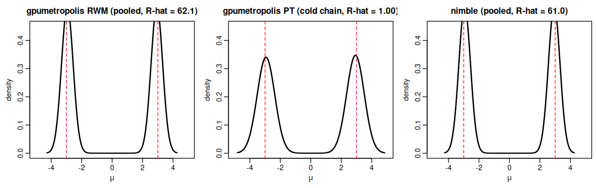
The three pooled densities look almost identical, two peaks at the reference modes. The difference is in the titles. R-hat near 1.00 for parallel tempering says the cold chain crossed; R-hat near 62 for the random-walk panel says each chain stayed in its starting basin. The peaks of the tempered run are slightly broader because that chain is actually sampling the spread inside each mode, not pinned to a point. The traces tell the same story without any summary statistic:
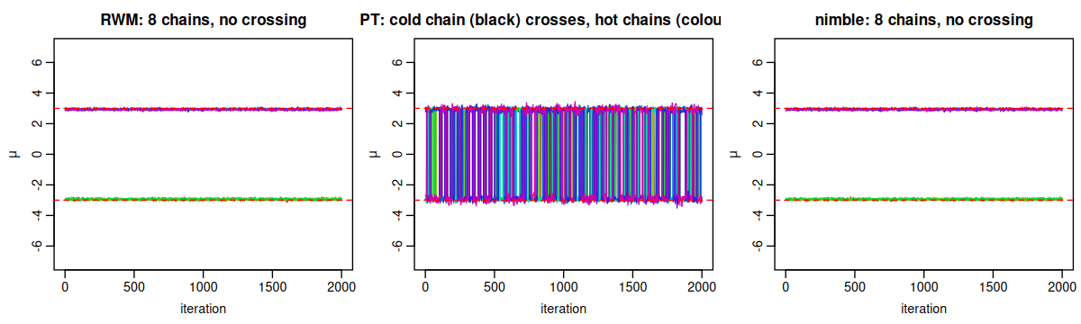
The eight random-walk chains are flat lines at +3 and -3, with no visible crossing across two thousand post-warmup iterations. The parallel-tempering cold chain, in black at the centre, jumps between basins the whole time, fed by the hot chains that mix freely on their tempered targets.
A focused re-run with twenty replications puts numbers on the cost, and adds the strongest competitor for this model, nimble, to the comparison.
| adapter | R-hat | ESS | ESS/s | wall-clock (s) |
|---|---|---|---|---|
| gpumetropolis (RWM) | 62.28 | 3525 | 27782 | 0.13 |
| gpumetropolis (PT) | 1.00 | 671 | 3007 | 0.23 |
| nimble | 61.97 | 3652 | 26973 | 0.15 |
Two readings stand out. First, nimble, with R-hat near 62, falls into the same trap: its eight chains stay in their basins too. The trap is a property of random-walk samplers on separated modes, not of one package. Second, the correct answer is not free. Parallel tempering pays a 1.7 times wall-clock factor for the host-side swap step, and reports a lower nominal effective sample size, because each cold-chain draw now carries the autocorrelation of a true mode-crossing chain rather than the false, low autocorrelation of a stuck one. The high ESS of the random-walk run is a number computed on a sample that does not represent the posterior. A converged R-hat at one fifth the nominal ESS is worth more than a large ESS at R-hat 62.
The honest rule of thumb: a unimodal target with moderate contrast is well served by the default random walk with adaptive warmup. Parallel tempering earns its cost when the posterior is multimodal with modes separated by low-density regions that random walk cannot cross within the iteration budget.
Part 2: where it bites, real extreme-value data
The toy was built to separate the modes cleanly. The reason to care is that a standard problem in applied statistics produces the same geometry without being asked to.
The setting is block maxima. Each year contributes its maximum, and under the classical theory the series of annual maxima is modelled as a Gumbel or a Generalised Extreme Value distribution (Coles, 2001). When a site sits at the edge of two climatic regimes, the same series carries two families of extremes, say summer-driven and winter-driven maxima, and a single Gumbel is then the wrong model. The posterior of the mixture that is the right model is multimodal, and the sampler from Part 1 is the one the problem needs.
A real dataset on the boundary
The evd::oxford series records annual maximum temperatures at Oxford from 1901 to 1980. Hartigan’s dip test for unimodality lands right on the conventional boundary:
diptest::dip.test(as.numeric(oxford))
#> D = 0.05625, p-value = 0.0531
#> alternative hypothesis: non-unimodal, i.e., at least bimodal
A p-value near 0.05 is the tie zone: the test neither clearly rejects unimodality nor comfortably accepts it. The sensible policy is not to pick one by fiat. It is to fit both candidates, a single Gumbel and a two-component Gumbel mixture, and let an information criterion such as WAIC choose. The single Gumbel is straightforward, in gpumetropolis or in the established evd::fgev maximum-likelihood route, and the two agree on the location near 83 Fahrenheit and the scale near 4.2 within a posterior standard deviation. The diagnostic panel of gpum_diagnose(fit_single) shows the full convergence picture in one glance:
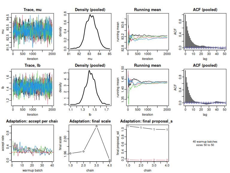
mu and lb = log(beta). Four chains overlap, R-hat sits at one, the effective sample size matches the iteration budget, and the marginals look like clean normals. The single Gumbel passes every test a unimodal posterior is supposed to pass.Two reasons the mixture is hard
That clean baseline is exactly what makes the Oxford mixture hard, and it is hard for two separate reasons. The first is specific to this dataset. With overlapping modes and only eighty points, the mixture posterior on (p, mu_1, beta_1, mu_2, beta_2) is weakly identified: the data can be reasonably explained by a single Gumbel, so the posterior has a wide ridge where one component dominates and the other becomes a “ghost” whose parameters drift through low-density parameter space. Extra structure is the principled fix, default priors and an order constraint on the locations plus posterior-predictive WAIC ranking, which is the design of the catalogue layer of v0.6.0.
The second reason is structural and holds for any mixture, however much data there is. A two-component Gumbel mixture has a log-density of the log-sum-exp form, log(p * f1(y) + (1 - p) * f2(y)), which the package’s formula DSL handles through log, exp and +. Every parameter is mapped to the real line so the sampler can propose freely, the mixing weight through a logit, the scales through their logarithm, the locations left unconstrained.
model_mix <- gpum_model(
  loglik = ~ log(
      (1 / (1 + exp(-eta_p))) *
        exp(-((y - mu1) / exp(lb1)) - exp(-((y - mu1) / exp(lb1)))) / exp(lb1)
    + (1 - 1 / (1 + exp(-eta_p))) *
        exp(-((y - mu2) / exp(lb2)) - exp(-((y - mu2) / exp(lb2)))) / exp(lb2)
  ),
  params = c("eta_p", "mu1", "lb1", "mu2", "lb2"),
  data   = "y"
)

fit_mix <- gpu_metropolis(model_mix, data = list(y = y),
                          init = init, n_iter = 8000, n_chains = 8,
                          method = "pt")
The two components can switch labels, component one and component two trade places, with no change in the likelihood, so the posterior has at least two equivalent labellings. That is the same separated-mode geometry of Part 1, and parallel tempering is again the right sampler; a canonical labelling, mu1 < mu2, is enforced in post-processing.
Recovering the mixture where it is identifiable
To see the mixture work without the ghost of weak identification, a small two-regime simulation isolates the problem in a setting where both components are identified. Each year is drawn from a cool-extreme Gumbel, mean near 22, or a warm-extreme Gumbel, mean near 36, with a mixing weight of 0.65 in favour of the warm component. The empirical sample is what such a station would actually produce, a histogram with a broad shoulder rather than two clean peaks:
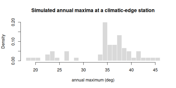
The tempered mixture fit on this simulation recovers all four Gumbel parameters within a posterior standard deviation, with the mixing weight slightly underestimated, the usual signal that for n = 60 the data identify the modes but not their exact balance. The cleanest visual check is posterior predictive: draw n_years new annual maxima from the posterior of the fitted mixture and compare the empirical distribution of those samples against the observed data.
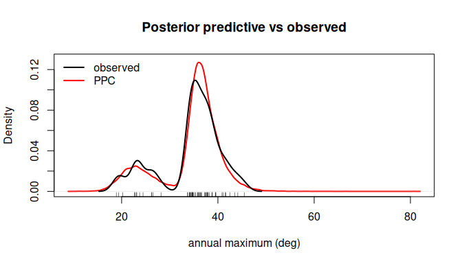
The mixture is therefore where the difficulty, and the value, sits.
The missing tool in R
The reason this is worth a package is that the mixture has no standard one-line tool in R today.
| Path | What it covers | Effort |
|---|---|---|
evd, extRemes, ismev, eva |
single Gumbel / GEV / GP | low, mature |
evmix |
bulk-and-tail hybrids | low for those families, not a Gumbel mixture |
mclust, mixR, flexmix, mixtools |
finite mixtures, almost only Gaussian | needs custom Gumbel density |
evdbayes |
Bayesian single GEV via Metropolis | manual extension for mixtures |
custom rstan / cmdstanr |
any coded mixture, including Gumbel | Stan code, label-switching, warm-up tuning |
custom nimble |
same with BUGS-style syntax | custom distribution, and, as Part 1 showed, the default sampler is trapped here |
Against that landscape gpumetropolis offers three things: one-formula declaration, the same R expression the user would write for the log-likelihood; built-in parallel tempering, the textbook tool for the label-switching multimodality, as method = "pt"; and one kernel source that runs on the CPU, CUDA and Vulkan, which matters when the series is long or the chains are many.
This is also where the package connects to a longer line of work on bimodal extremes. The bimodal Gumbel distribution itself, a single distribution for two-mode extreme behaviour, was studied in bgumbel (Otiniano, Brom and others, 2023, Austrian Journal of Statistics), on CRAN. The mixture route here and the single bimodal-Gumbel route there are two answers to the same applied question, and a forthcoming catalogue layer in gpumetropolis v0.6.0 will collapse the fit-and-compare workflow to a single call, gpum_fit_catalog(y, catalog = c("gumbel", "gumbel_mix2"), ranking = "WAIC").
Where the GPU fits, and where it does not
None of the above needs a GPU; the Oxford series has eighty points, and on a series that small the CPU backend is faster than the GPU, because there is no data-parallel work to amortise the kernel launch. The GPU axis of gpumetropolis pays off in a different regime, many chains or an expensive log-density over a large dataset, and the package documents that plainly rather than promising unconditional speedups. The registered benchmark against the established R MCMC packages makes the regime explicit.
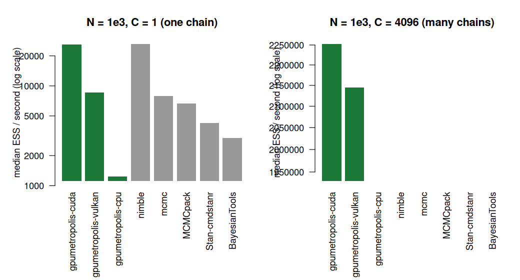
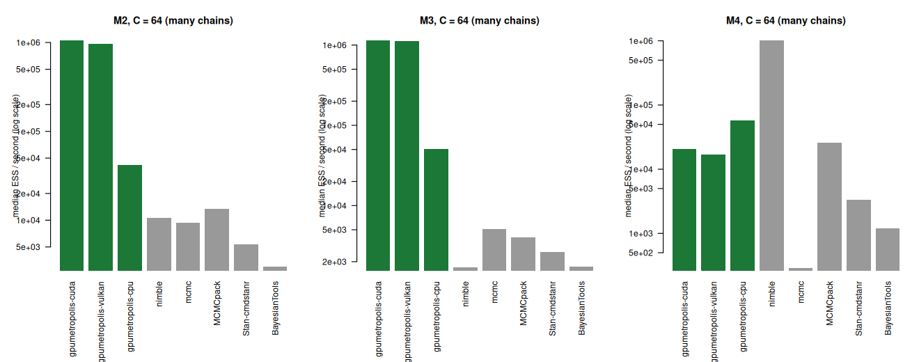
With one chain the package does not beat a mature CPU sampler. With many chains it inverts: on the heavy-tailed model it reaches 225 times the best competitor at 64 chains, and at 4096 chains it is the only backend that completes the cell at all. On the conjugate Gaussian it loses to nimble, which detects the structure and draws directly, and the package states that loss as plainly as the wins. The full design, the six pre-registered hypotheses with their support and refutation conditions, and the per-cell numbers are frozen in the package’s EXPERIMENT_PROTOCOL.md, committed before any result existed.
The lesson, and the toolkit
The pooled density is the wrong place to look for convergence on a multimodal target. It is built from the same draws whether the chains mixed or stayed stuck, and on a symmetric problem it looks correct in both cases. The split R-hat is the diagnostic that separates the two, and a value far above one is a refusal, not a caution. When it fires on separated modes, parallel tempering is the fix, at a wall-clock cost that buys an answer that is actually the posterior. And the geometry is not exotic: a two-regime extreme-value mixture, a common situation at a climatic edge, carries it by construction, and the mixture has no one-line tool in R today.
The package is open source and under active development; the worked cases above are the first two chapters of its living companion, alongside the heavy-tailed and ill-conditioned models of the registered benchmark. The code, the protocol and the vignettes are at github.com/pcbrom/gpumetropolis, installable from R-universe.
References
- Coles, S. An Introduction to Statistical Modeling of Extreme Values. Springer, 2001.
- Hartigan, J. A., and Hartigan, P. M. The dip test of unimodality. The Annals of Statistics, v. 13, n. 1, p. 70-84, 1985.
- McLachlan, G., and Peel, D. Finite Mixture Models. Wiley, 2000.
- Otiniano, C. E. G., Brom, P. C., and others. The bimodal Gumbel distribution. Austrian Journal of Statistics, 2023. DOI 10.17713/ajs.v52i2.1392.
- Stephenson, A. G. evd: Extreme value distributions. R News, v. 2, n. 2, p. 31-32, 2002.